Download this worksheet as a .Rmd
Getting familiar with R
Aim of this worksheet
After completing this worksheet, you should feel comfortable typing commands into the R console (or, REPL) and into an R Markdown document. In particular, you should know how to use values, variables, and functions, how to install and load packages, and how to use the built-in help for R and its packages.
Values
R lets you store several different kinds of values. These values are the information that we actually want to do something with.
One kind of value is a number. Notice that typing this number, either in an R Markdown document or at the console, produces an identical output
42## [1] 42- Create a numeric value that has a decimal point:
Of course numbers can be added together (with +), subtracted (with -), multiplied (with *), and divided (with /), along with other arithmetical operations. Let’s add two numbers, which will produce a new number.
2 + 2## [1] 4- Add two lines, one that multiplies two numbers, and another that subtracts two numbers.
Another important kind of value is a character vector. (Most other programming languages would call these strings.) These contain text. To create a string, include some characters in between quotation marks "". (Single quotation marks work too, but in general use double-quotation marks as a matter of style.) For instance:
"Hello, beginning R programmer"## [1] "Hello, beginning R programmer"- Create a string with a message to your instructor.
Character vectors can’t be added together with +. But they can be joined together with the paste() function.
paste("Hello", "everybody")## [1] "Hello everybody"Mimic the example above and paste three strings together.
Now explain in a sentence what happened.
Another very important kind of value are logical values. There are only two of them: TRUE and FALSE.
# This is true
TRUE
## [1] TRUE# This is false
FALSE## [1] FALSENotice that in the block above, the # character starts a comment. That means that from that point on, R will ignore whatever is on that line until a new line begins.
Logical values aren’t very exciting, but they are useful when we compare other values to one another. For instance, we can compare two numbers to one another.
2 < 3## [1] TRUE2 > 3## [1] FALSE2 == 3## [1] FALSE- What do each of those comparison operators do? (Note the double equal sign:
==.)
- Create your own comparisons between numeric values. See if you can create a comparison between character vectors.
R has a special kind of value: the missing value. This is represented by NA.
NA## [1] NATry adding 2 + NA.
- Does that answer make sense? Why or why not?
We will come back to missing values.
Variables
We wouldn’t be able to get very far if we only used values. We also need a place to store them, a way of writing them to the computer’s memory. We can do that by assignment to a variable. Assignment has three parts: it has the name of a variable (which cannot contain spaces), an assignment operator, and a value that will be assigned. Most programming languages use a rinky-dink = for assignment, which works in R too. But R is awesome because the assignment operator is <-, a lovely little arrow which tells you that the value goes into the variable. For example:
number <- 42Notice that nothing was printed as output when we did that. But now we can just type nummber and get the value which is stored in the variable.
number## [1] 42It works with character vectors too.
computer_name <- "HAL 9000"No output, but this prints the value stored in the variable.
computer_name## [1] "HAL 9000"- In the assignment above, what is the name of the variable? What is the assignment operator? What is the value assigned to the variable?
Notice that we can use variables any place that we used to use values. For example:
x <- 2
y <- 5
x * y
## [1] 10x + 9## [1] 11- Explain in your own words what just happened.
Now create two assignments. Assign a number to a variable and a character vector to a different variable.
Now create a third variable with a numeric value and, using the variable with a numeric value from earlier, add them together.
Can you predict what the result of running this code will be? (That is, what value is stored in a?)
a <- 10
b <- 20
a <- b
a- Predict your answer, then run the code. What is the value stored in
aby the end? Explain why you were right or wrong.
Vectors
Variables are better than just values, but we still need to be able to store multiple values. If we have to store each value in its own variable, then we are going to need a lot of variables. R is a beautiful language because every value is actually a vector. That means it can store more more than one value.
Notice the funny output here:
"Some words"## [1] "Some words"What does the [1] in the output mean? It means that the value has one item inside it. We can test that with the length() function
length("Some words")## [1] 1Sure enough, the length is 1: R is counting the number of items, not the number of words or characters.
That would seem to imply that we can add multiple items (or values) inside a vector. R lets us do that with the c() (for “combine”) function.
many <- c(1, 5, 2, 3, 7)
many
## [1] 1 5 2 3 7- What is the length of the vector stored in
many?
Let’s try multiplying many by 2:
many * 2## [1] 2 10 4 6 14- What happened?
- What happens when you add
2tomany?
Can you create a variable containing several names as a character vectors?
Hard question: what is happening here? Why does R give you a warning message?
c(1, 2, 3, 4, 5) + c(10, 20)## Warning in c(1, 2, 3, 4, 5) + c(10, 20): longer object length is not a
## multiple of shorter object length## [1] 11 22 13 24 15Built-in functions
Wouldn’t it be nice to be able to do something with data? Let’s take some made up data: the price of books that you or I have bought recently.
book_prices <- c(19.99, 25.78, 5.33, 45.00, 22.45, 21.23)We can find the total amount that I spent using the sum function.
sum(book_prices)## [1] 139.78Try finding the average price of the books (using
mean()) and the median price of the books (usingmedian()).Can you figure out how to find the most expensive book (hint: the book with the maximum price) and the least expensive book (hint: the book with the minimum price)?
Hard question: what is happening here?
book_prices >= mean(book_prices)## [1] FALSE TRUE FALSE TRUE FALSE FALSEUsing the documentation
Let’s try a different set of book prices. This time, we have a vector of book prices, but there are some books for which we don’t know how much we paid. Those are the NA values.
more_books <- c(19.99, NA, 25.78, 5.33, NA, 45.00, 22.45, NA, 21.23)- How many books did we buy? (Hint: what is the length of the vector.)
Let’s try finding the total using sum().
sum(more_books)## [1] NA- That wasn’t very helpful. Why did R give us an answer of
NA?
We need to find a way to get the value of the books that we know about. This is an option to the sum() function. If you know the name of a function, you can search for it by typing a question mark followed without a space by the name of the function. For example, ?sum. Look up the sum() function’s documentation. Read at least the “Arguments” and the “Examples” section.
- How can you get the sum for the values which aren’t missing?
Look up the documentation for ?mean, ?max, ?min.
- Use those functions on the vector with missing values.
Data frames and loading packages
We are historians, and we want to work with complex data. Another reason R is awesome is that it includes a kind of data structure called data frames. Think of a data frame as basically a spreadsheet. It is tabular data, and the columns can contain any kind of data available in R, such as character vectors, numeric vectors, or logical vectors. R has some sample data built in, but let’s use some historical data from the historydata package.
You can load a package like this:
library(historydata)- The dplyr package is very helpful. Try loading it as well.
You might get an error message if you don’t have either package installed. If you need to install it, run install.packages("historydata") at the R console.
We don’t know what is in the historydata package, so let’s look at its help. Run this command: help(package = "historydata").
- Let’s use the data in the
paulist_missionsdata frame. According to the package documentation, what is in this data frame?
We can print it by using the name of the variable.
head(paulist_missions, 10)## mission_number church city state
## 1 1 St. Joseph's Church New York NY
## 2 2 St. Michael's Church Loretto PA
## 3 3 St. Mary's Church Hollidaysburg PA
## 4 4 Church of St. John Evangelist Johnstown PA
## 5 5 St. Peter's Church New York NY
## 6 6 St. Patrick's Cathedral New York NY
## 7 7 St. Patrick's Church Erie PA
## 8 8 St. Philip Benizi Church Cussewago PA
## 9 9 St. Vincent's Church (Benedictine) Youngstown PA
## 10 10 St. Peter's Church Saratoga NY
## start_date end_date confessions converts order lat
## 1 4/6/1851 4/20/1851 6000 0 Redemptorist 40.71435
## 2 4/27/1851 5/11/1851 1700 0 Redemptorist 40.50313
## 3 5/18/1851 5/28/1851 1000 0 Redemptorist 40.42729
## 4 5/31/1851 6/8/1851 1000 0 Redemptorist 40.32674
## 5 9/28/1851 10/12/1851 4000 0 Redemptorist 40.71435
## 6 10/19/1851 11/3/1851 7000 0 Redemptorist 40.71435
## 7 11/17/1851 11/28/1851 1000 0 Redemptorist 42.12922
## 8 12/1/1851 12/8/1851 270 0 Redemptorist 41.79854
## 9 12/10/1851 12/19/1851 1000 0 Redemptorist 40.27979
## 10 1/11/1852 1/22/1852 600 3 Redemptorist 43.04485
## long
## 1 -74.00597
## 2 -78.63030
## 3 -78.38890
## 4 -78.92197
## 5 -74.00597
## 6 -74.00597
## 7 -80.08506
## 8 -80.20982
## 9 -79.36559
## 10 -73.63007(The head() function just gives us the first number of items in the vector.)
That showed us some of the data but not all. The
str()function is helpful. Look up the documentation for it, and then run it onpaulist_missions.Also try the
glimpse()function.Bonus: where does the
glimpse()function come from?
We will get into subsetting data in more detail later. But for now, notice that we can get just one of the colums using the $ operator. For example:
head(paulist_missions$city, 20)## [1] "New York" "Loretto" "Hollidaysburg" "Johnstown"
## [5] "New York" "New York" "Erie" "Cussewago"
## [9] "Youngstown" "Saratoga" "Troy" "Albany"
## [13] "Detroit" "Philadelphia" "Philadelphia" "Cohoes"
## [17] "Wheeling" "Cincinnati" "Louisville" "Albany"Can you print the first 20 numbers of converts? of confessions?
What was the mean number of converts? the maximum? How about for confessions?
Bonus: what was the ratio between confessions and conversions?
Plots
And for fun, let’s make a scatter plot of the number of confessions versus the number of conversions.
plot(paulist_missions$confessions, paulist_missions$converts)
title("Confessions versus conversions")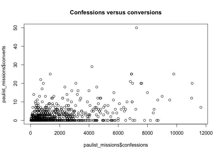
- What might you be able to learn from this plot?
- There are other datasets in historydata. Can you make a plot from one or more of them?